SeaTac

Seattle's (relatively) cool winter, Part 1...

Updated on April 6, 2023


I first published this blog post on March 18. The day before,  it warmed to the 60’s for the first time since October in and around Seattle. This felt very nice to my cold bones. It has been a relatively cool winter this year if you look at the December – February traditional winter period. January was relatively mild, warm, and dry for a winter period in Seattle. But the traditional meteorological winter was bookended by a coolish December and February. Extend the bookends of the period to November and March (to-date), four of the past five months have been cooler than normal.

My charts only contained data through March 15 when I first published the post on March 18. Now, a week into April, I have data through the end of March. The updated figures below reflect this.

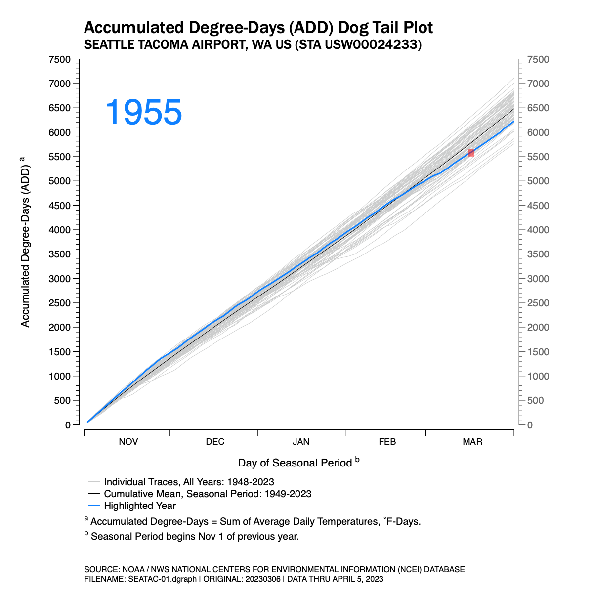
I’ve posted several charts below. Figure 1 is an animation. The chart is a series of traces which track the cumulative average daily temperature recorded at Seattle Tacoma International Airport (KSEA) for the seasonal period of November 1 through March 31 for the years 1949 through 2023.

NOTE: The animation is an animated GIF file programmed to loop through twice. Each loop takes roughly 25 seconds. Refresh the browser window (command+R) to restart the animation.

Figure 1. Accumulated daily average temperature traces by seasonal year, 1949-2023, at Seattle Tacoma International Airport.

A few notes about Figure 1 follow:

  1. I’ve chosen a “made-up” metric. I don’t know if this is used by the National Weather Service, meteorologists, or climatologists with any regularity. I call my metric or index the Accumulated Degree-Day (ADD). It simply takes the average daily temperature recorded at KSEA and adds it to the previous days. It is similar to Heating Degree-Days and Cooling Degree-Days which are commonly summed over a period of time but my ADD does not use a threshold temperature of 65˚F to compare against. But it does give one an idea of how cool or warm the seasonal period has been in comparison to similar periods in other years at a common location.  I suppose it’s units would be ˚F-Days.

  2. The gray traces in the background display each year from 1949-2023 for an aggregate comparison.

  3. A blue trace is highlighted for each individual year as the animation is played.

  4. Since each seasonal period plotted crosses two calendar years, I’ve chosen the latter of the two calendar years to identify each individual trace. So, the trace for the November 2022 – March 2023 period is identified as ‘2023.’

  5. The highlighted blue traces extend to March 31 for each year.

  6. An average ADD trace for all years has been added to the chart for comparison. The ADD trace is shown as a black  hairline. For the total November–March season period, the total average ADD value is 6482 ˚F-Days.

  7. Some data went uncollected by the National Weather Service on March 16-17, 2023 at Seattle Tacoma International Airport which made it difficult to calculate a daily Average Daily Temperature for these dates. The missing data is explained in the chart and the days impacted are shown in a red block on the chart.

  8. Finally, I name the animation a dog tail chart because when played back, especially at higher frame rates, these types of charts look a little like a wagging dog tail. 


So why an animation? Animations display motion, and motion display movement over time and, possibly, patterns. You may want to ask yourself; year-to-year is there any rhythm, pattern or trending that becomes obvious that might be difficult to discern when comparing a series of still images or charts. This is especially true when comparing 74 still images if each chart was published separately (and they are further below).

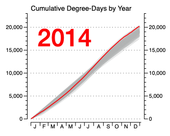
 And there does appear to be some patterns at the distal ends of this period we’re investigating. In the late 40’s and through the mid-1950’s there are a series of coldish winter seasons(7 of 9 between 1949-1957). This is well documented in old photographs of heavy snows in Seattle during this period. And one could argue that the 2010’s have a pattern of warmer than normal winters (6 of 8 between 2014 through 2021). But mostly, this animation shows the high level of variance fluctuating between cooler-normal-warmer winter cycles. The late 2010’s may have shown warmer periods, but this season is quite cooler. And there were warmer winter seasons in the 1950s.

*****

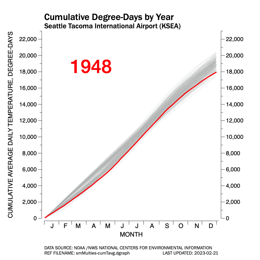
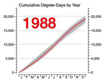
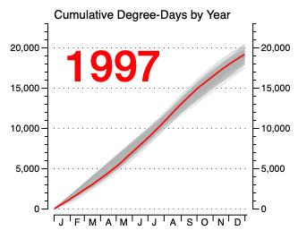
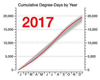
The individual annual temperature traces which make up the animation are shown below. The are shown in order of the earliest year (1949) to the most current (2023). Click on any individual image below to see more detail and to compare.

Temperature changes at SeaTac...

Weather data collected at Seattle Tacoma International Airport (SeaTac) is generally considered the main data of record for the Seattle metropolitan area, though there are several other sites in the region where meteorologist and climatologists gather their information. Data has been collected at SeaTac continuously since 1948, though some data is missing from the records for the period of October 1, 1996 through October 31, 2005. This missing data is generally the snow and sky cover observations. Temperature, the focus of this page, and precipitation data was collected during this period and is available from the National Oceanic and Atmospheric Administration (NOAA) and their publicly accessible National Centers for Environmental Information (NCEI) Climate Data Online (CDO) tool.

So, having temperature data from 1948 through yesterday (Feb 22, 2023), how much has the average daily temperature changed at SeaTac over the past 75 years (inclusive) if at all? And are there any trends? If so, one would assume that the temperatures have slowly warmed over the years based on all the science and reporting published over the past decade or longer.


An undulating plot

The National Weather Service generally reports the daily minimum temperature (Tmin) and daily maximum temperature (Tmax) at the weather stations. The average of these two values is calculated and recorded as the average daily temperature (Tavg). Often when looking at or downloading past data from a weather station, the user receives only the Tmin and Tmax values for a given date. This is common on older records. Sometimes the data includes the calculated Tavg. Regardless, knowing that Tavg is the average between the Tmin and Tmax values, the Tavg shown in the following charts has either been calculated by the NWS and reported, or this author has performed the calculation in the spreadsheet I’ve imported data from the NWS into.

If you plot the TAVG value for every date from January 1, 1948 through today as shown in Figure 1 you get an undulating or wavy curve form. Obviously, the average daily temperature of a summer day is much higher than the same on a winter day in Seattle. It is difficult to determine if there has been a fall or rise in the average daily temperature and, if so, by how much by just looking at this wave form.

Figure 1. Average daily temperatures trace from 1948 to 2022, Seattle Tacoma International Airport.

I’ve added a linear trend line in red in Figure 2. This trend line shows a modest rise in daily temperatures over the 75-year period. The average daily temperature recorded at Seattle Tacoma Airport has risen from roughly 50˚F to about 54˚F during this period, a rise of roughly 4-4.5 ˚F, or 2.2-2.5 ˚C.

Figure 2. Average daily temperatures trace from 1948 to 2022 with red trendline, Seattle Tacoma International Airport.

Annual Cumulative Degree-Day Index (ACDD)

Another method of looking at temperature changes over time and comparing these to other years over a long period is to plot the cumulative total of daily average temperatures and plot that accumulation over the course of a year. Then plot a similar curve for each year in the period of study. This is shown in Figure 3.

A simple way to check this value is described here. Say the average annual daily temperature at SeaTac is 50˚F. This is the average daily temperature over the course of a year. Some days will be cooler and some warmer. If you multiply (50F DEGREES) X (365 DAYS) you’ll get a value of  18,250 DEGREE-DAYS, or 18,250 DD. I’ll use the term Annual Cumulative Degree Day (ACDD) to indicate the degree-days accumulated over an annual period at a specific weather station.

Looking at the y-scales on Figure 3 shows that summing the average daily temperatures for each day of the year will get you to approximately 18,250 ACDD.

Note: My use of an index I call degree-day is not the equivalent of Heating Degree Days (HDD) or Cooling Degree Day (CDD), both indexes used in the building systems world to calculate required heating or cooling loads for designing heating and air-conditioning equipment and systems and both reported on in daily summary statistics from NOAA/NWS data repositories. But it is similar in the sense of understanding the total amount of heat received over the course of a year (as defined by the sum of the daily average temperatures) in any given year at SeaTac airport. Each gray line or trace shown in Figure 3 represents one year in the 1948-2023 period.

Figure 3. Annual Cumulative Degree Days (ACDD) plots for each year, 1948-2022, Seattle Tacoma International Airport (KSEA).


Comparing individual years

Figure 4 shows ACDD traces of four individual years (highlighted in red) plotted against similar ACDD traces all years. Of the four selected, 1948 and 1985 started off relatively cool through the end of June and then each had a cool autumn and early winter. The plot for 1966 shows it too started cool through spring and into early summer before a late summer surge gave it a relatively average ACDD Index value for the entire year. The plot for 2015 shows the year had an average winter and spring temperature-wise for this region, followed by a warm period extending through the remainder of the year. For the 74 full years between 1948-2022, this year (2015) was the warmest on record in Seattle.

Figure 4. Individual ACDD trace samples for four select years, Seattle Tacoma International Airport.


Small Multiples

Figure 5 is a series of plots grouped as a whole. Each individual plot can be clicked on to expand it. This form of data graphic is collectively called small multiple. It allows one to compare one year to other years easily. It also allows for a deeper dive into any individual year.

Detecting trends requires a little more study, but you can see that, in generally, the ten years from 1948-57 were cooler than average at SeaTac. One can also see that the 10-year period from 2013 through recently completed 2022 have been warmer than average. There was another five-year period running from 2003-07 which were warmer than average. Most of the other years hovered near average, though it is common over any ten year stretch to see back-to-back years running much cooler or warmer than average.

Figure 5. A small-multiples data graphic comparing the Annual Cumulative Degree Days (ACDD) tracing for each of 74 consecutive years at Seattle Tacoma International Airport.

Another interesting thing that shows up when plotting the Degree-Day number for each year is best seen going back to Figure 3. Notice how in the winter and early spring months, Seattle tends toward either warmer or cooler springs. Very few annual periods are “average”. Notice the “gap” that exists between early February through May. This period in the calendar tends towards two groups or strands of tracings which braid together in midsummer. By the end of each calendar period, the tracings have advanced towards split ends.

I don’t know why. I wonder if La Nina years tend towards one strand and El Nino years towards the other. Mathematicians, meteorologists, or atmospheric scientists might understand this “strand” phenomenon or “strand theory” better than I.


An Animated Chart

Finally, Figure 6 is an animated chart. It is an alternative to the small multiples chart shown in Figure 5. It displays each year’s trace above the gray traces of all years sequentially. You can imagine it looking like a dog’s tail wagging. This means of presenting data highlights the year-to-year variability. It also can show trends if over a course of periods of years, the “tail” wags high or lower. You can witness by watching the video the early years of recorded temperatures tend towards cooler days and as time marches forward, the wagging tail inches up the chart. Year-to-year the tail wags randomly (annual variability), but over time a pattern emerges of the tail drifting upwards into warmer cumulative temperatures (periodic trending).

Figure 6. ACDD traces for Seattle Tacoma International Airport, 1948-2023. The animated GIF should loop through once, probably upon initial loading of the web page. Notice that the wagging red line slowly drifts higher as the years progress. Drifting high indicates the total daily temperature load is increasing (e.g. days are getting warmer on average).

HINT: Refresh (Command+R) the web page to cycle the GIF in sequence. And remember to scroll back down to the bottom of the page after refreshing.


That’s all for this post, just some interesting new ways at looking at annual temperature profiles for data from selected NOAA / NWS collection sites. I used SeaTac Airport as an example as I live in Seattle.

Rearview Mirror: November 2021

The November 2021 Temperature Departure chart is shown in Figure 1.

In general we’ve had a somewhat cooler than normal autumn, but November was slightly warmer than normal, with a monthly temperature average of 47.9˚F, about 1.4F above normal. Several strong atmospheric storms hitting the Puget Sound region from the tropics to the southwest passed through the city mid-month and towards the end. These storms brought warm, tropic air with them with plenty of moisture. These multi-day temperature spikes can be seen in Figure 1.

Figure 1. Daily temperature departs from 30Y climatic normals through November 30.

Click image to enlarge.

Normally, I’d add a chart showing new monthly precipitation totals, but I’ve reported these in several previous blog posts over the past few days. There’s no sense repeating that information here. Click to Prev button at the bottom of this post to navigate to those posts if you’re interested.


DATA SOURCE
NOAA / National Weather Service Local Climate: https://www.weather.gov/wrh/climate?wfo=sew

Nooksack flooding, 2021

It has been a rainy start to autumn in Seattle in 2021. Figure 1 shows a plot of the cumulative precipitation at Seattle-Tacoma (SeaTac) International Airport since the beginning of the 2021-22 water year. Water years in Seattle are date-based construct starting on October 1st and running through September 30 of the following year. These are often used when discussing precipitation events since the west coast of North America and specifically the Pacific Northwest of the U.S. can often be divided into a wet season (late fall through early spring) and a dry season (late summer through early autumn).

The plot below highlights the current water year precipitation accumulation but also includes similar traces for all water years at SeaTac since 2002-03. Compared to recent years, this year – just starting – is quite wet.

Click on any figure below to expand it.

Figure 1. Cumulative rainfall, Seattle-Tacoma International Airport, current water-year. Also show are traces from previous water-years, 2002-03 through 2020-21.

Figure 2 highlights on of the past two decades wettest start to winter for comparison purposes. This was the 2006-07 water year. November of that month registered close to 15.6 inches of rain.

It has not been nearly as wet this November with roughly 8 inches of precipitation so far, about two-thirds of the way through the month. But if you compare the two lines on the chart, Seattle has had a much wetter October in 2021, so the total precipitation to date is similar between the 2006-07 and 2021-22 water years.

Figure 2. Comparison of current water-year cumulative precipitation with the 2006-07 water-year trace.

Figure 3 shows an additional year with a very wet start, the water year of 2016-17. This wet year reached approximately the same total precipitation as 2006-07 for the two-month, OCT-NOV period, a value of roughly 17 inches total. Normal precipitation totals for Seattle-Tacoma for that two-month period is typically about 10 inches. In the 2021-22 water year, with November still one week away from completing, we have seen 13.66 inches of rain since October 1.

Figure 3. Current water-year cumulative precipitation at SeaTac Airport with the 2006-07 and 2016-17 precipitation traces highlighted.

Figure 4 is a little bit different than the first three charts. I often track weather out of SeaTac. But I rarely step out to track weather in other areas, even areas not so far from home. Last week, in the northwestern part of Washington State and in southern British Columbia, large volumes of rain, arriving in the form of an atmospheric river, flooded the region. The flooding was quite severe, impacting many homes and farms, and creating great havoc and damage to many roads and highways. Many people were stranded by the flood waters and needed to be rescued. Several people have died in this storm.

I’ve plotted the cumulative rain totals recorded at the Bellingham International Airport since October 1. Bellingham is a mid-sized city approximately 90 miles north of Seattle, and very close to the flood zone. In fact, parts of Bellingham were under water for several days after these recent storms.

In Figure 4 you can see the total amount of rain falling in Bellingham has been very similar to that of SeaTac. Until about November 8, Belingham was tracking about 2 inches less in rain compared to Seattle from the start of the new water year. But from November 9-15, Bellingham received approximately 6.6 inches of rain, about 2.5 inches more than Seattle in that week.

I regularly keep track of these precipitation vs. time charts for Seattle-Tacoma International Airport. Adding Bellingham totals to the chart was only for comparison reasons only. Inthe most recent storm, it’s likely the Seattle area was protected to some extent by the Olympic Range to our west. Bellingham is not as well protected.

Figure 4. For comparison purposes, this figure shows the current year precipitation trace at Bellingham International Airport with the past 20 year traces at Seattle-Tacoma International Airport. Note: Bellingham is approximately 90 miles north of Seattle.


The United States Geological Service (USGS) keeps track of river flows across the country. Some of this data is exposed to the public. Two gaging stations the USGS keeps near the Whatcom County flood zone are the stations on the Nooksack River at Everson and at Ferndale. Everson is about 12 miles ENE of Ferndale as the crow flies. The monitoring station at Ferndale appears to have records published over a much longer time period, so this data will be used for comparison purposes. The Nooksack river flows from the Mount Shuksan and Mount Baker watersheds. On the other hand, the station at Everson, also on the Nooksack, is much closer to the Sumas River which presumedly caused much of the flooding in the Fraser River Valley in British Columbia.

The Nooksack river major flood stage at Ferndale is 23 feet. The Nooksack river crested above this stage on November 16 (Figure 5, lower chart) at 23.7 feet.

Figure 5. Nooksack River stage charts from Ferndale WA from November 15-22, 2021. Chart is courtesy of the USGS.

Figure 6. Nooksack River stage charts from Everson, WA from November 15-22, 2021. Chart is courtesy of USGS.

Table 1 shows the values of historic stage crests on the Nooksack River at Ferndale for crests above 12.25 feet. The values were copied into this table from the source listed below the table. I entered the most recent value (blue entry) for 11/16/2021 since the web site values had not been updated yet.

This November’s flood stage ranked with the top twenty events at this gage site.

Table 1. Record gage levels for the Nooksack River at Ferndale WA. Source: NOAA / NWS.

Source link

Figure 7 is a dot plot of the historic crests on the Nooksack River at Ferndale ordered from great to least. Color coding indicate the decade of the event.

Figure 7. A dot plot showing the historic flood stages on the Nooksack River at Ferndale WA.

Figure 8 is a series of dot plots of the same data as shown in Figure 7. The data has been grouped in decades to see if any trends can be found due to time. Decades are an arbitrary grouping. But often we group data in years, decades and centuries to see patterns time-related data, so I used decade groupings here.

I don’t see any obvious patterns in the decade groupings other than some early decades had fewer but more severe events and more recent decades had more events but events which appeared less severe in terms of gage height. Of course, the 2020s are just beginning. It is possible, I suppose, that less severe events in the early 1910-30 period were not as diligently recorded. And it might also be true that less severe events in more recent decades may do more damage due to greater populations and development in the area. These are just guesses.

Click on any chart to enlarge. You can use left and right arrow keys to navigate between decadal sets of data.

Figure 8. A series of dot plots of ordered historic crests on the Nooksack River at Ferndale WA grouped by decade. Click to enlarge.


Figure 9 shows the data in Table 1 in a time-series chart format (which is basically a horizontal dot plot sorted by time rather than rank).

Again, strong patterns are hard to find, other than the first half of the timeline tends to show greater historic crests. I don’t know the reasons for this. Maybe storms were stronger in the past. Perhaps physical river control methods have been installed over the years to help regulate flow. Since 1965, it is difficult to discern any distinct pattern to the historic crests other than every 15 years or so, a moderate-high or major flood event occurs.

Figure 9. Time-series chart of historic crests on the Nooksack River at Ferndale, WA.


Finally, it should be noted that parts of northern Whatcom County and much of the Fraser River Valley were flooded and not on the Nooksack River, but rather on the Sumas River. The Nooksack flows west to Puget Sound from the North Cascades. The Sumas River flows north into Canada. The U.S. border town of Sumas was severely flooded the past week as was much of the nearby Fraser River Valley.

There is a point near Everson, WA where the Nooksack river runs very close to the Sumas River. The surrounding land is generally flat. Literature suggests past overflows of the Nooksack have flowed into the Sumas near Everson. The distance appears to be less than two miles at the closest points

I suspect this is what happened this past week. I’m not a hydrologist, so I don’t really know. But with all of the water falling last week and the weeks leading up to this event, it seems likely. River gage data on the Sumas for the public was difficult to find.

Figure 10 shows the proximity of the two rivers. Directionally, north extends into the top background in the image.

Figure 10. Proximity of the Nooksak River to the Sumas River. Image courtesy of Google Earth. Click to enlarge.

The Bellingham Herald is the paper of record in Whatcom County and Northwest Washington. The paper has excellent coverage of the recent floods and photo essays of past historic floods. Flooding in this region is not uncommon. It is a flat landscape at the base of very steep mountains subject to heavy winter rains and runoffs.


FULL DISCLOSURE

I am not a meteorologist, climate scientist, data scientist, geologist nor hydrologist. I am simply a (retired) engineer who has some familiarity with numbers, basic statistics and probability statistics who enjoys looking at readily available public data and trying to make sense of things. I enjoy building data visualizations from data I find much like others enjoy working daily crosswords or sudoku puzzles. Local weather, climate and hydrology science are complex subjects. Take what you read and find here with this in context.

Seattle-Tacoma's hottest days...

Charts updated: August 14, 2021, 8:00 AM PDT

We’re in the midst of a second heat wave this summer. Our first, in late June, was a scorcher, setting an all time high record for Seattle at Seattle-Tacoma International Airport (SeaTac) on June 28 of 108˚F. We had three days of temperatures greater than 100˚F in that period.

This week’s heat wave (and now smoke wave) isn’t quite as hot. But temperatures are back above 90˚F. This is a arbitrary threshold, but it is as good as a threshold for a heat wave as any, so we’ll use it.

****

So, how often does it get to 90˚F or greater in Seattle, The Land of No Air-Conditioning? It is pretty much a summer only phenomena and is not as uncommon as one might think. Figure 1 shows maximum daily temperatures at SeaTac going back to January 1, 1949. Most summers record at least one or more days of 90˚F, but not all. This year is about average. We’re not through with this current heat wave, so one can expect to see another red dot for today and probably tomorrow. I can’t predict beyond tomorrow whether we will see anymore really hot days. But it is becoming late summer. Days are gradually getting shorter and nights longer and we only have about 2-½ more weeks until September begins.

Ironically, in the six or so weeks between this summer’s heat waves, we’ve had one of the most pleasant, if a bit dry, summers in my 38 years here.

Click on Figure 1 to expand it. I’ll update it over the next few days as this heat wave plays itself out.

Figure 1


Figure 2 was added on August 14. It shows a zoom-in of Figure 1 for the last 10 years. Most summers in Seattle experience at least a few days with temperatures reaching 90˚F.

Figure 2 also shows the extraordinary heat wave Seattle experienced in June 2021 where temperatures exceeded 100˚F for three straight days.

Figure 2


© itterrocks.com, 2021.. All rights reserved.
Please contact litterrocks via the Contact link in the lefthand margin for permission to use.

Tags: Tmax, maximum temperatures, weather, Seattle-Tacoma International Airport, KSEA, summer, heat